You are probably wondering if the title is clickbait. It is not. Check out the short video clip below for a pretty convincing demo.

The speedup¹ is highly dependent on the data, and for the two traces shown it is 33× and 22×. But 30× is a nice round number, and it is in the range of what you can reasonably expect here.

How is this possible? (tl;dr version)

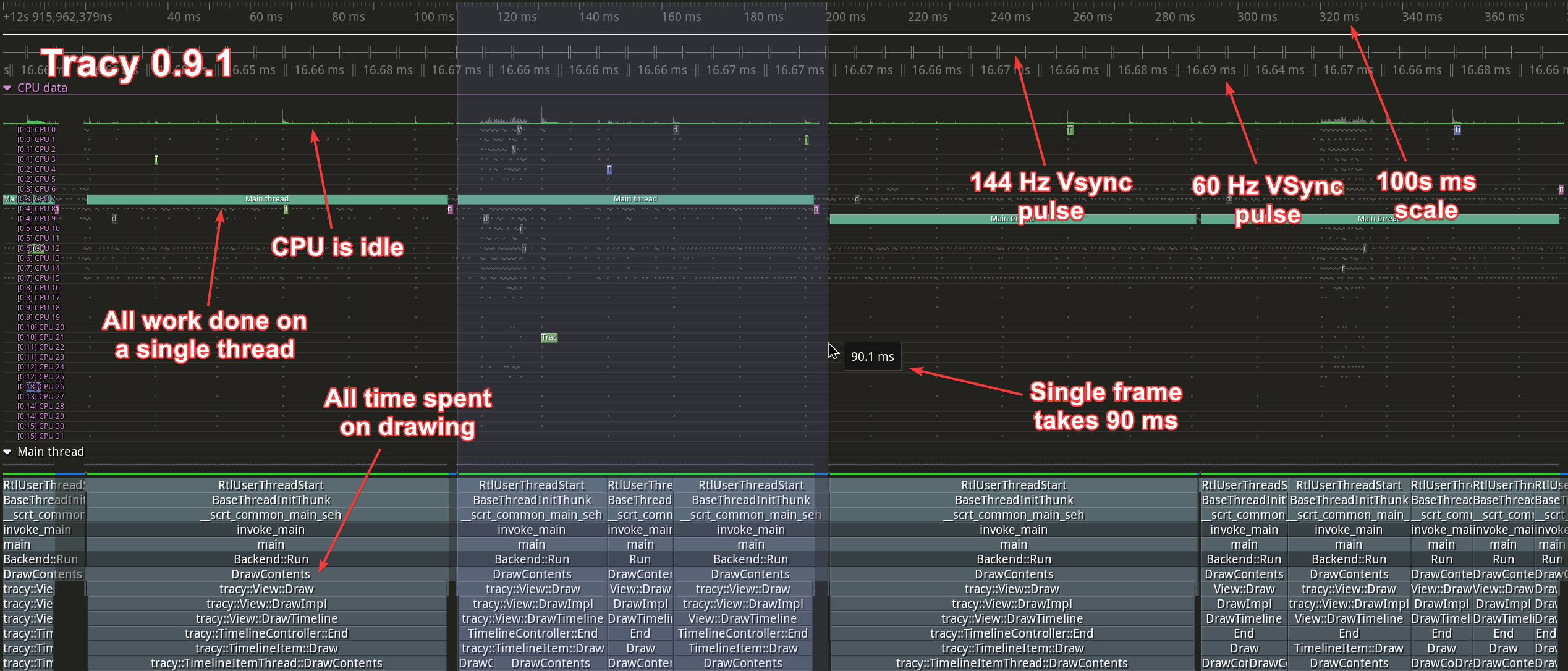
We can use Tracy to profile itself² to be able to easily see where the change is. Here’s what happened before:

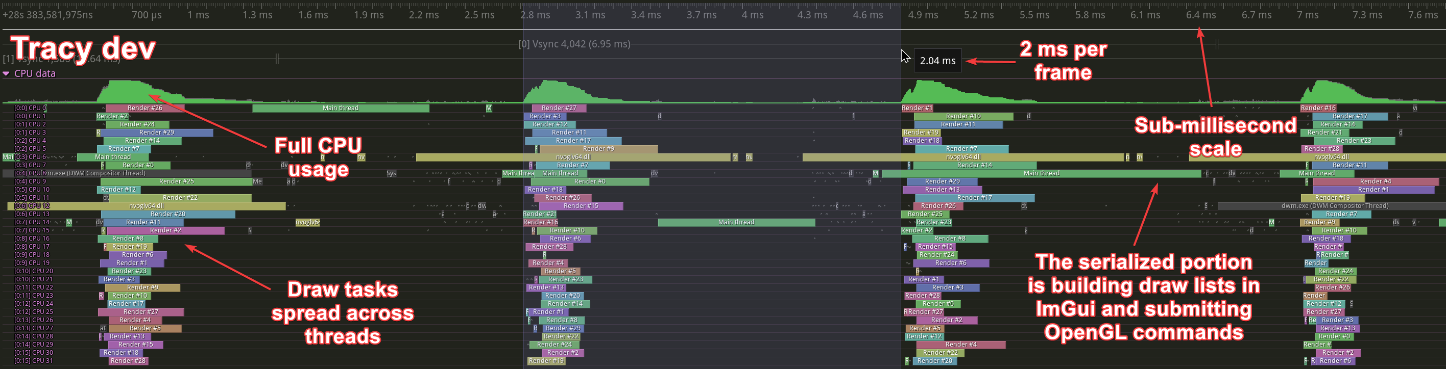
And here is what it is doing now:

You may have noticed that the speedup here is 45×. This is because a different zoom level was used than in the video above, and the amount of data to be processed has changed.

What happens there?

To render the timeline view, Tracy must first figure out what needs to be drawn. This is done by performing binary searches on large amounts of data. A binary search accesses memory at “random” locations, and it is not possible to predict where the next access point will be, so things like prefetching don’t work here³. If each step of the search makes round-trips to system memory instead of working within the cache, the CPU does very little work because it is constantly waiting for data.

Typically, when you’re working with Tracy, you won’t have that much data to process, and you won’t notice any slowdown. If you have 10 zones visible in a thread (a number you can comfortably work with), and each of those zones has no more than a few children, the search scope will probably fit completely in the cache and everything will be fast. This has actually proven to scale quite well to even larger numbers, probably because the memory access patterns don’t change that much between each step, so the hot search path can remain largely in the cache.

If you have hundreds of millions of zones to manage⁴, things can get slow. However, this all depends on what you need to display on the screen. Zoom in too close, and you only have to deal with the few zones that happen to be in view. Zoom out too far, and now you have to calculate content just for a few columns of pixels where the data actually is. But zoom in just right, and now you have to search your entire dataset, and you have to do it for every column of the 4K screen you might be using.

Once you have figured out what to draw, you have to actually draw it on the screen. Tracy uses ImGui to prepare the vertex buffers that are later passed to OpenGL.

Storing the data

Tracy is very efficient in the way it stores data. For example, a CPU zone is described by the following structure:

struct ZoneEvent
{
    uint64_t _start_srcloc;
    uint16_t _child2;
    uint64_t _end_child1;
    uint32_t extra;
};

The total data size is 22 bytes⁵, of which the start and end timestamps occupy 6 bytes twice⁶, 2 bytes are the source location index, and there are two 4-byte indexes for child vector reference and the optional extra data storage. Keep in mind that if you are storing a billion zones, adding even one additional byte to this data structure will increase the memory requirements by 1 GB.

It would make no sense to track each of these small data structures individually, and you need to process them one at a time as they arrive from the profiled application. To handle this, Tracy allocates 64 MB blocks of memory and writes data to them sequentially. There is no way to erase anything.

The type of data you have to write to memory is semi-random in nature. You might be processing a zone start event, then you might have to process a lock event, which is immediately followed by a bunch of plot items. There are no context-specific memory pools in use, everything ends up in the same memory buffer. Note that this is true for a live capture. You will get slightly better data grouping if you load a trace from a file on disk, due to the way things are stored.

Another memory optimization is the use of 6-byte pointers. On current 64-bit hardware, you cannot operate in the full 64-bit address space. You are limited to 48 bits⁷. Tracy exploits this by providing a short_ptr pointer type.

While these optimizations are introduced to conserve memory, they have the added benefit of increasing cache locality, simply by packing more data into the same limited space.

Searching the data

We know the time at the start (left) and end (right) of the screen for each timeline view configuration. This is stored in m_vd.zvStart and m_vd.zvEnd. To find out the range of ZoneEvents within a data array that are visible on the screen, we can do two quick searches⁸:

auto it = std::lower_bound(vec.begin(), vec.end(), m_vd.zvStart,
    [] (const auto& l, const auto& r) { return l.End() < r; });
const auto zitend = std::lower_bound(it, vec.end(), m_vd.zvEnd,
    [] (const auto& l, const auto& r) { return l.Start() < r; });

Now that we know what the boundary elements are, we need to iterate over what is visible:

while(it < zitend)
{
    const auto end = it->End();
    // pxns converts nanosecond values to on-screen pixels
    const auto zsz = (it->Start() - end) * pxns;
    if(zsz < MinVisSize)
    {
        // nspx converts on-screen pixel values to nanoseconds
        const auto MinVisNs = MinVisSize * nspx;
        int num = 0;
        const auto px0 = (it->Start() - m_vd.zvStart) * pxns;
        auto px1ns = end - m_vd.zvStart;
        auto rend = end;
        auto nextTime = end + MinVisNs;
        for(;;)
        {
            const auto prevIt = it;
            it = std::lower_bound(it, zitend, nextTime,
                [] (const auto& l, const auto& r) { return l.End() < r; });
            if(it == prevIt) ++it;
            num += std::distance(prevIt, it);
            if(it == zitend) break;
            const auto nend = it->End();
            const auto nsnext = nend - m_vd.zvStart;
            if(nsnext - px1ns >= MinVisNs * 2) break;
            px1ns = nsnext;
            rend = nend;
            nextTime = nend + nspx;
        }
        const auto px1 = px1ns * pxns;

        // Draw collapsed zones on screen, handle tooltips, etc
        // ...
    }
    else
    {
        if(it->HasChildren())
        {
            DispatchZoneLevel(it->Child());
        }

        // Draw zone on screen, handle tooltips, etc.
        // ...

        ++it;
    }
}

We will not analyze this code, but I will point out a few things:

• The function of this code is to group together zones that are too small to display. It does this by looking for zones that fit into the MinVisSize region (3 pixels) from the end of the last processed zone.
• We are working in the time domain and in the pixel domain, and there is no clear boundary between them.
• The code searches for what needs to appear on the screen and then immediately proceeds to draw it. Mixing two different operations is not good for the performance of either one. They step on each other’s toes in terms of resource usage.
• It’s hard to understand what’s going on.

Improving the way things are

The solution, as spoiled at the top of the page, is to parallelize everything you can. Why would you want to process everything on a single thread when you have all those CPU cores sitting around doing nothing at all? If you know you will be waiting for a lot of time, you can just wait for multiple things at the same time.

Now, how would you divide up the tasks to be done? What are the indivisible units? Let’s take a look.

Each arrow points to a completely separate task to be computed. For example, you can’t split the processing of CPU zones within a thread because they are hierarchical, but you can easily process two different threads at the same time. Similarly, thread properties such as messages, samples, context switches, or locks (which are not shown in the picture) are not dependent on each other and can be computed simultaneously.

In addition, the search algorithm is now separated from the drawing logic and does not have to compete for limited CPU resources. The result is improved performance. Better code clarity is the icing on the cake. Compare the code below with the code above. It is much easier to understand.

while(it < zitend)
{
    const auto end = it->End();
    const auto zsz = end - it->Start();
    if(zsz < MinVisNs)
    {
        auto nextTime = end + MinVisNs;
        auto next = it + 1;
        for(;;)
        {
            next = std::lower_bound(next, zitend, nextTime,
                [] (const auto& l, const auto& r) { return l.End() < r; });
            if(next == zitend) break;
            auto prev = next - 1;
            const auto pt = prev->End();
            const auto nt = next->End();
            if(nt - pt >= MinVisNs) break;
            nextTime = nt + MinVisNs;
        }
        m_draw.emplace_back(...);
        it = next;
    }
    else
    {
        if(it->HasChildren())
        {
            PreprocessZoneLevel(it->Child());
        }
        m_draw.emplace_back(...);
        ++it;
    }
}

The m_draw array contains descriptions of things to be drawn later. Typically it won’t contain more than a thousand elements. The data stored in it is quite simple, and it just closely follows what is needed on the other side.

enum class TimelineDrawType : uint8_t
{
    Folded,
    Zone,
    GhostFolded,
    Ghost
};

struct TimelineDraw
{
    TimelineDrawType type;
    uint16_t depth;
    short_ptr<void*> ev;
    Int48 rend;
    uint32_t num;
};

It’s only 20 bytes and covers not only the manually instrumented CPU zones, but also the ghost zones generated from the sampling data.

The draw data for other elements can be even simpler. For example, here’s the data structure for thread context switches:

struct CpuCtxDraw
{
    uint32_t idx;
    uint32_t num;
};

The drawing logic is also much more straightforward now. It only needs to iterate over the draw list and perform dispatch on different things to draw:

for(auto& v : drawList)
{
    switch(v.type)
    {
    case TimelineDrawType::Folded:
        ...
    case TimelineDrawType::Zone:
        ...
    case TimelineDrawType::GhostFolded:
        ...
    case TimelineDrawType::Ghost:
        ...
    }
}

And that’s basically it.

What has made this optimization possible?

I have known about the performance issues when viewing large amounts of data for a long time. So why was this only fixed now?

The “clean code bad” rant by Casey Muratori. It sparked some discussion that led to Jason Booth’s “Practical Optimizations” video. It is a good talk and worth watching. There was nothing really new for me in it, but it did manage to plant an intrusive desire in me to try parallelization. Inspiration works in strange ways sometimes.

Well, it’s just parallelization, it’s not hard, right?

It is very hard.

The whole performance vs. clean code discussion started at the end of February. It’s almost May now. I’ve been working on it all the time.

I had no idea if this would even work. It could have turned out that the concurrent memory accesses would have blocked each other out.

I seriously considered parallelizing the ImGui draw command submission. I wrote some prototype code to do this. Separating the search logic from the drawing logic was a scary concept. I was not sure if accessing the randomly scattered data during drawing would be fast enough. I did not know how much data would have to be stored between the search and draw phases. This applies both to the number of entries in the draw lists and to the data in the entries themselves.

It was hard to figure out what the original search logic was doing. I had to sit down with a piece of paper and a pencil and think about it all over again and rewrite the whole thing.

Then I had to do it again and again, because every little search I have is basically tailor-made to support some obscure need. The CPU zones have to be hierarchical, you have to include children. The locks, like most things in Tracy, can be collapsed if there are too many to draw within a couple of pixels. But the contended areas of the locks must be visible, even when you zoom out! Otherwise, you’re hiding key data. Or what about plots that may need to compress millions of plot elements down to a few pixels wide, but still retain the general shape of the plot?

Finally, there are all the new bugs to fix. And in the end, most users won’t even see a difference in Tracy’s performance because they only work with small traces, and the tool was already fast enough!

So it may look easy in retrospect. But it was not. And getting the idea that it might be beneficial was the hardest part.

Additional opportunities

Another optimization that I was able to squeeze in is a change in the way things are drawn. As you know, when items are too small to fit on the screen in Tracy, they are replaced by a zigzag pattern. Previously, this pattern was drawn by issuing path stroke commands to ImGui. The library generated the geometry for the line segments, making sure that each segment was properly attached to its neighbors. All these calculations were quite visible when profiling, so a replacement was in order. This is especially true since the invocation of ImGui is now a large part of the application that still needs to be serialized.

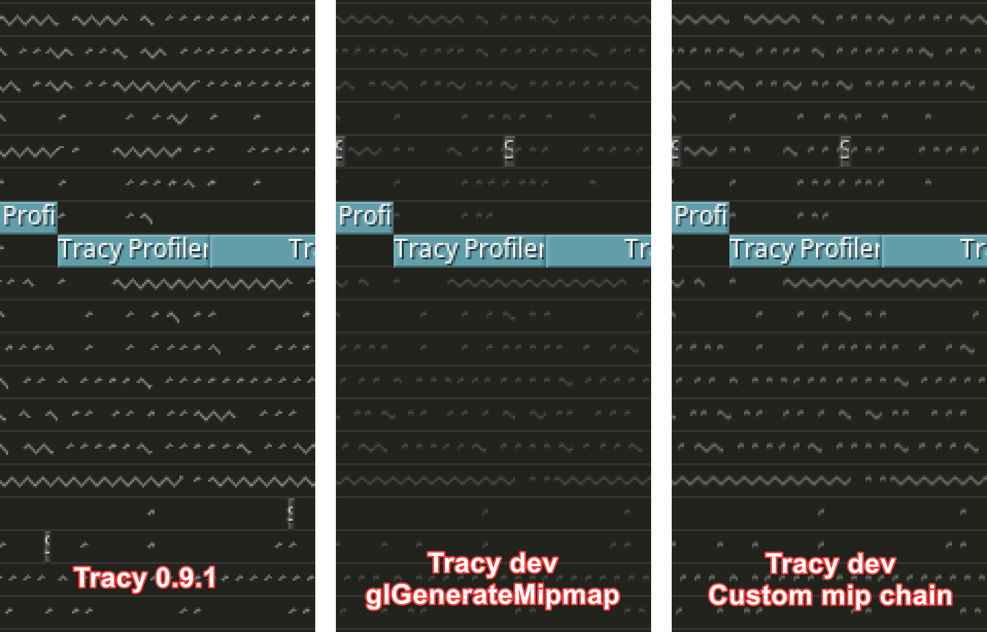
Simple enough! Just fire up Inkscape or something and draw the pattern. Then load it and use it as a texture instead of doing the strokes. Since the zigzags can be very small, we’ll also use glGenerateMipmap to avoid aliasing artifacts. And we’re done, right?

Well, of course not. What works okay at 32 or 16 pixels high will blend too much with the surrounding transparency when squeezed down to 2 or 4 pixels. Everything will look too dark. So now you have to prepare the entire mip chain by hand, making the stroke bolder and bolder as you scale it down, so that it maintains that ideal width of 1 pixel at every size. See the results below.

Note that drawing with the old method still made things look sharper. Of course, there are remedies for this. You can create the zigzag pattern on the fly, in the exact sizes you need, to avoid any scaling and the associated blurriness. Or you can leave everything to shader math. But such solutions aren’t what I’m interested in at the moment.

The final bummer is that this new drawing method, while taking considerably less time in the profiling statistics, reduces the framerate. My guess is that the CPU is now so underutilized that it does not need to increase its operating frequency as much as before. Such is the fun of code optimization.

Update #1 (2023-05-01)

The day after I wrote this blog post, I added an option to limit the number of search threads to just one. And then I had to check if everything was working correctly because it was hard to notice any slowdown⁹. The non-threaded rendering is able to reach about 10 ms frame times. This may not be enough to reach 144 Hz refresh rates, but it’s not too bad either.

It turns out that the main performance driver was apparently the separation of the search phase from the ImGui draw submission phase. The exact speedup is hard to determine because the new search algorithm, while generally following the old one, was rewritten from scratch.

A long time ago I wrote a software renderer that basically did the same lighting as the Dope demo by Complex back in 1995. The relatively simple 3D model had a detailed object space normal map. You would then rotate the normal vectors to account for model motion and use the resulting values to sample a 2D texture with baked-in lighting. This was a primitive form of image-based lighting.

To make it work on slow hardware (the Nokia N73 had a 220MHz ARM processor with no FPU), you had to use a lookup table. One that you indexed with the normal map color value (which was 16-bit because you had to fit everything into about 10 MB of RAM), and which would give you the color to write to the screen.

My first approach was to be reasonable and calculate only what was necessary. The basic algorithm was to check if the current normal vector value was already handled, and if not, to do all the necessary calculations in the middle of rendering a triangle.

I also tried another approach. I calculated all 64K lookup table values before rendering. This was complete nonsense, because half of the table would never be used, since backwards facing triangles are never rendered.

The second solution was significantly faster.

So, going back to the profiler’s behavior, I’d say I’m surprised, but not confused.